Using New Technology to Study Climate Change
As science and technology continue to advance, the ways in which scientists and engineers study the surface of the Earth and how it will change in the future, changes along with it. The field of climate change science is continuing to benefit as advances in technology lead to a greater understanding of how climate changed in the past and create new ways to generate more high-resolution data sets of current Earth systems.
One example of how scientists and engineers are combining these advances in technology with high-resolution data sets is through the creation of computer generated simulation models. These are computer programs that are designed to simulate past or future events. Computer models are used in many different scientific fields, including astronomy, economics, physics, biology, geology, etc. One type of computer model that most people are familiar with are atmospheric models that are used in weather forecasts. Climate change scientists also use computer models to simulate how the Earth will be affected due to the effects of global warming and the rise of greenhouse gases in the atmosphere. These models try to predict outcomes such as future temperature rise, changes in weather patterns, risk to coastal cities, likelihood of future droughts, etc.
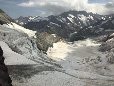
The extent of future sea-level rise due to climate change is one of the biggest unknowns in the field of climate science. Teams of scientists across the world are working on creating swaths of data and complex computer models to unravel this problem. However, large uncertainties in the parameters used in some of these sea-level models still exist. One of the largest uncertainties in sea-level predictions is the contribution of water from the melting of mountain and continental glaciers. This is due to the fact that the principles that govern the flow of a glacier down the slope of a mountain or landscape, known as “Sliding Laws”, are highly variable based on the data used to calculate the rates. One of the unknowns in this data is how the shape of the land beneath a glacier affects its melting rate and subsequent contribution to sea-level rise. Ongoing research in the Swiss Alps and other worldwide locations is attempting to address this issue by generating high-resolution field data from current glacial locations (Figure 1).
Before real world landscapes like the one shown in Figure 1 can be incorporated into computer modeled simulations, scientists and engineers must figure out a way to turn this space into data that can be understood by a computer. A picture of these areas is not sufficient, as it does not contain detailed information on the height, geographic location, etc. The landscape would need to be built in the computer, similar to the way backgrounds or scenery is built in video games or computer generated movies and graphics. Furthermore, this data would need to be extremely accurate in order to build the best computer model possible for the simulation.
There are currently three different methods that scientists and engineers can use to convert a 3D landscape into usable and accurate data, and they are outlined below.
Method #1- The Emery Method
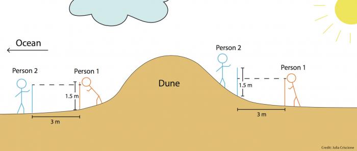
The simplest method to digitize a landscape, or take systematic measurements of a landform in order to create a profile of the land, is the Emery Method (1961). This low-tech method involves two people systematically moving two, 1.5 meter long sticks, separated by a fixed distance along a predetermined profile of the landscape. Data is collected along the profile as the two measuring sticks move up or down relative to each other (Figure 2). This method has been used extensively to create beach profiles, but can also be used to measure any landscape. The Emery Method is very inexpensive but can be very labor-intensive when trying to capture the shape and variations in very rugged or complex terrain. There is also the high probability that much of the variation in the terrain will be lost or not captured due to the low-resolution nature of this measurement technique.
Method #2- Ground and Aerial Based LiDar
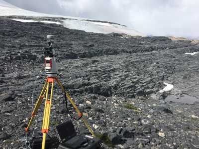
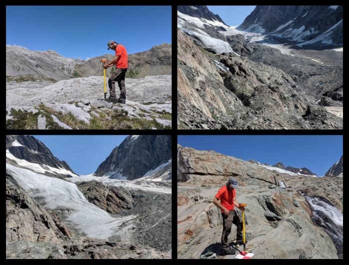
The word Lidar, also known as LIDAR, LiDAR, and LADAR, is now used as an acronym of “light detection and ranging”. This refers to the surveying technique that uses measured wavelengths and return times of a pulsed laser source between an object and a sensor to measure distance (Figure 3). These distances can then be used to create digital 3D representations of an object. The mathematical principles behind this method are very similar to sonar or echolocation, i.e., the way submarines navigate and bats fly, respectively. Lidar is often referred to as 3D laser or 3D scanning and was originally used by the National Center for Atmospheric Research to measure clouds. The process can detect ultraviolet, visible, or near-infrared light and is therefore useful for targeting a wide range of objects and materials, such as rocks, rain, chemical compounds, aerosols, clouds, or even single molecules. Lidar has numerous practical applications, and has been used for mapping the surface of the moon, predicting agricultural crop yield rates, creating high-resolution digital elevation models of geologic and archaeological sites, helping to guide autonomous vehicles, creating conservation maps of forests, mapping fault zones, scanning buildings or formations to make 3D models (Figure 4), measuring greenhouse gas emissions, and much, much more.
For more information on LiDar, visit this website.

Method #3- Structure from Motion

Structure from motion (SfM) is a computer program that estimates distances of a three-dimensional structure from a series of two-dimensional images. To calculate the SfM, point or feature correspondence must be determined between a series of images. This process computes a fundamental matrix and uses the corresponding points found in the previous step for the computation. This matrix is then uploaded to the “relativeCameraPose” function to determine the orientation and location of the camera's point of view in the different photographs. The 3D locations are then determined by triangulating the matched points. This process will create the correct shape of the structure, but it will not be scaled to the actual size. The scale of the structure can be determined by adding additional information into the program, such as GPS coordinates, or allowing the program to detect an object of known size within the structure.
SfM has many applications, such as 3D scanning, augmented reality, environmental and landform studies, etc. (Figure 5). The SfM program is particularly useful in the geosciences when studying remote locations that are difficult to access or traverse, or when rough terrain might cause a loss of data or image foreshortening. Although ground-based lidar techniques provide higher-resolution data than the SfM program, these methods are very labor-intensive and time-consuming. However, SfM can generate a data cloud that is comparable in accuracy and density to those generated by airborne lidar techniques, often at a fraction of the cost. This method has been applied in a variety of settings, including rivers, coastlines, fault zones, cliffs, and coral reefs.
- For more information on the SfM program, visit this website.
Sliding Glaciers and Forefields in the Swiss Alps
The data presented in this activity was collected as part of the National Science Foundation funded project “Collaborative research: Development of sliding laws for glacier-flow and landscape-evolution models” and the PolarTREC project, “Sliding Glaciers”. As part of this project, a team of researchers spent 18 days in the Swiss Alps collecting data from drone-based aerial photography of former glacier beds. The SfM program was then used to take these images and convert them into 3D models of the exposed glacier beds. These models are used in computer simulations that will help scientists develop better sliding laws for glaciers or the rate at which glaciers slide down a mountain. This, in turn, will help scientists to better constrain the uncertainties in future sea-level rise due to the melting of mountain- and land-based glaciers. Even though this field site is not located in a polar region, the work done here will improve models of ice sheet flow relevant to polar regions.

Because glaciers act as big bulldozers, they are usually pushing a bunch of rock and debris at the front end or terminus of the glacier. When the glacier begins to retreat, it will leave this debris at the point of its maximum growth. Geologists call this pile of rock and debris a terminal moraine. The terminus, or outer edge/tongue of the glacier is always changing, but the area of land between the terminus and the terminal moraine is called the forefield (Figure 6).
The goal of this field work was to create high-resolution 3D images of several glacial forefields in the Swiss Alps. The 3D printed model used in this activity was created from thousands of aerial drone photographs of the Upper Lang glacial forefield in Switzerland during the summer of 2018 (Figure 7). To learn more about how this field work was done, please visit the “Sliding Glaciers” blog.
Objectives
Lesson Preparation
By the conclusion of this activity, the goal is for students to have been introduced or learn the following concepts.
Have a basic understanding of the various ways scientists digitize landscapes to turn a 3D terrain into data.
How recent advances in technology, such as drones and computer algorithms, are advancing our knowledge of the Earth and making it easier to acquire data.
How new technology can help address some of Earth’s major environmental issues, like climate change.
Without scientists and engineers working together, studies like this would not be possible.
Creation of 3D Printed Models
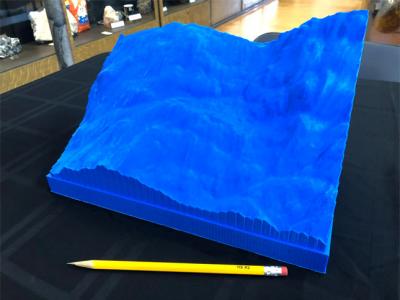
The 3D prints were created from high-resolution aerial photographs that were acquired with a drone. The 2D drone images were then imported into the SfM program to create a 3D image. This process is explained in detail below in the section titled “Downloading and Using Structure from Motion”. After running the SfM program, a .psx file, or Metashape Project file of the 3D image will be created. Some SfM programs, like the one we used (i.e., the Agisoft Metashape program), will allow you to export the image as an .obj file. If this is not an option, additional programs, like QGIS, can be used to convert the .psx file to an .obj.
The Sliding Glaciers team partnered with the Rutgers Makerspace to further modify the 3D models to make them more durable and easily manipulated for teaching purposes. The 3D models were modified in Autodesk Inventor to add a base and additional features to assist in the laboratory procedure. Once the models were finalized, they were exported into an STL format, a standard format for 3D printing slicing software, which prepares the machine code for the 3D printers.
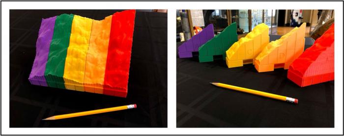
The following is a list of the 3D printing files that are available for download in the document section of this activity.
Ordering 3D Prints
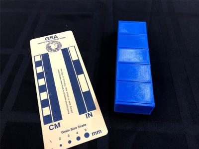
If you are not familiar with printing your own 3D models, the files provided here can be sent or uploaded to a number of companies that will make the prints for you. Many local universities and libraries also support their own “Makerspace” facility that will be equipped to help print and create these models.
Here is a list of companies that will 3D print files for you:
Settings for Printing Models on Your Own
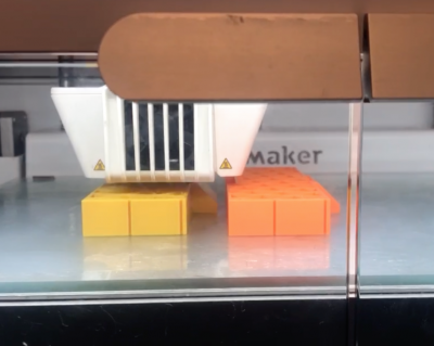
The models were printed on Ultimaker S5s, Ultimaker 3s, and Lulzbot Taz6s, all types of “FDM” 3D printers (Fused Deposition Modelling or Fused Filament Fabrication, “FFF”). When printing on the Ultimaker printers, we used the most recent version of CURA to slice and prepare the models to print. On the Lulzbot printer, we used an offshoot version of CURA maintained by Lulzbot specific to their printers. All printers were equipped with 0.4 mm nozzles and heated beds. However, a heated bed is not necessary to print PLA plastics.
The models were printed in PLA filament, with a 0.2 mm layer height and 10% infill and otherwise standard settings for each printer. PLA, or polylactide, is a biodegradable thermoplastic aliphatic polyester derived from renewable biomass, typically fermented plant starch. PLA is a very common 3D printing filament, is easy to achieve good results with and generally compatible with most FDM printers. Support structures are unnecessary, as the models are designed to be easily printed on FDM printers.
The models are scaled to be approximately 60 x 130 mm in the x and y planes and between 120 and 140 mm in the z plane. The size of the models allows them to be printed on smaller format printers. The models may be further scaled as needed if all models are scaled by the same percentage. The orientation of the models will place the bottom of the base directly on the print bed. They may be rotated in the xy plane to allow for placing additional models on one print bed, but it is recommended to keep the bottom of the base on the print bed when printing. The puzzle piece connections are chamfered by 45 degrees to ensure that no support structures are necessary.
The large model of the full scan is scaled to approximately 225 x 130 mm in the x and y planes and 140 mm in the z plane. This may be larger than the maximum print volume on some 3D printers. If the model is too large for a print bed, using the scale feature in the printer's slicing software to resize the model to appropriate dimensions will remedy the issue. Alternatively, the model may be scaled up to the maximum allowable print volume. There is no need for supports on the full model and it may be printed with standard print settings. Finally, the blocks used to display student work may be printed with standard settings and are small enough such that multiple blocks may be printed at a time.
Procedure
Introductory Discussion
Teachers should have read the introductory information provided in the sections above. Depending on the age and level of the students, the teacher can either provide them with copies of the above text to read on their own, or teachers can work through a guided discussion of the motivation for the study and the different methods used to turn landscapes into “data”.
Alternatively, that discussion can be bypassed and the activity can start with a brief class discussion on drones. Be sure to discuss what they are and how they can be used in science. This discussion can be supplemented with pictures and videos of drones from the internet. Small drones are relatively inexpensive, so drone demonstrations can also be conducted with the students.
Here are some articles on how drones are being used to advance knowledge across many scientific fields, including the geosciences.
- Drones in Geoscience Research: The Sky Is the Only Limit
- Thirteen Innovative Ways Humans Use Drones
- How Drones are Advancing Scientific Research
To complete the activity as described, teachers will need to obtain the materials listed below. Be sure to look over the section on printing the 3D model, as teachers and students will need access to at least one 5-section “printed 3D mountain puzzle” to complete this activity.
Examination of the 3D Models
Following the introductory discussion, give each group of students one set of “puzzle piece models”. Allow students to examine the models and ask them to make observations. Explain to students that these models were created through images taken from drones and that the shape and slope of the mountain they see in the 3D model is what the landscape looks like in the real world. This scaled model actually represents an area of land that is approximately 5 football fields in length.
The goal of the “Sliding Glaciers” project was to take an actual landscape and turn it into data that a computer can understand. The computer will then use this data to run simulations to test and examine various theories and scenarios to come up with estimates of the future effects of climate change.
Tell students to imagine they are standing on the actual mountainside and not just holding the model of the landscape. Ask them to think about how they could go about turning that landscape into data, e.g., height, latitude, longitude, etc. You can allow students to come up with their own methods or lead them through a discussion of the three methods that are outlined at the start of this lesson.
Below is a list of the take-home points you want students to walk away knowing after the discussion and hands-on activity.
- Advances in technology have helped scientists collect extremely accurate data about the Earth.
- Not only is the quality of the data improved with new technology, but the speed at which it can be collected has rapidly increased as well.
- Without technology like drones, the only way to collect this type of data would be to manually collect it by hiking throughout the landscape with measuring tapes and maps.
- When scientists and engineers work together, the speed of data collection can go from days to weeks (Emery method), to days (LiDar), to hours (Drones and SfM).
Activity Instructions
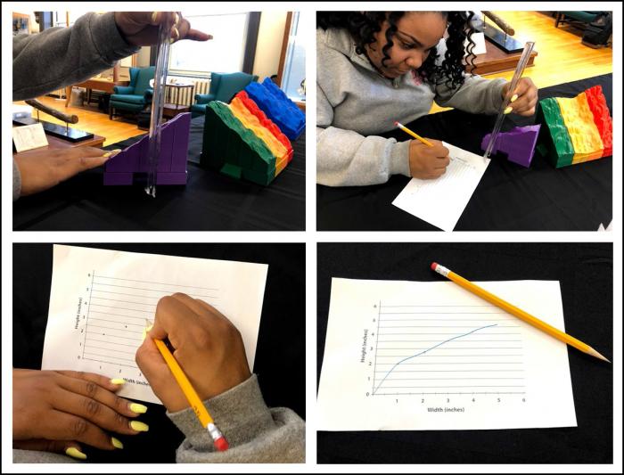
The following set of instructions will help teachers guide students through a simulation of the Emery Method of manually creating data profiles of a landscape. Please refer to Figure 12 for images of how these measurements will be taken.
After handing out the “puzzle piece” models to the students, have them look over each of the pieces. The sides of the models are lettered A to E and represent the surfaces where the students will be making the profile measurements.
Have students measure the height (y-axis) at several different locations along the x-axis. There are no units assigned to this part of the model, but they are spaced so that the lines are 1-inch apart. Students can take measurements at each of these intervals, or you can have them come up with their own points of measurement along the x-axis. The more measurements they take, the more accurate their profile will be. This is a point that can be addressed by comparing profiles between groups at the end of the activity.
Once all the measurements are taken on piece “A”, have the students plot their data points on a blank graph provided and connect the points to make a line graph. Label this graph letter “A”.
Repeat these steps for all remaining “puzzle pieces” and label these graphs B to E. Students can also measure the outer edges of the model (not labeled with letters) to create two more profiles and increase the accuracy of their data.
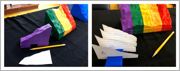
Once all of the profiles have been plotted onto the blank graphs, cut out the profile along the x-axis, y-axis, and along the line that was created by connecting the data points (Figure 13).
There should now be at least 4 pieces of paper that resemble the shape of your “puzzle piece” mountain model. Place these profiles into the base block in the correct order.
Create Your Own 3D Images
If time permits, teachers can use the SfM program to create their own 3D image from 2D photographs. Choose an item in the classroom or an outdoor landscape familiar to the students. Instructions on taking good photographs, downloading, and running the SfM program are provided below.
If this part will be used as a demonstration, the teacher must take all the photographs and run the SfM program ahead of the class to have it ready to show the students. A student project can also be created from this if the teacher asks the students to take their own pictures of an object or landscape. They will then be able to create their own 3D images. If time doesn’t permit, the internet can be used to show students pictures and/or videos of this program being used to digitize landscapes and a variety of other applications.
Reflection
Now is the time for students to make comparisons between the 3D printed model and the model they made using the Emery method. Spend some time discussing these differences and what process or factors could account for these differences. Have them reflect on the three methods of turning a landscape into data covered in the activity. Ask the students to list some benefits and drawbacks to each of the methods. Students should be able to explain how the science and technology are interrelated in this project. Have students think about other ways these methods and technologies could be used to study the Earth.
Assessment
No formal assessment has been designed for this activity, but rubrics could be developed by individual teachers to match their classroom needs. Students could also be asked to write a "5-minute Essay" describing what they learned by completing the activity.
Extension
By creating the data profiles of the mountainside, students will gain an appreciation and understanding of how modern technology has helped to further the field of science. Not only does technology allow for faster acquisition of more accurate data, but the use of drones will allow scientists to explore even more physically challenging terrain that may not have been accessible before.
Although optional, using the SfM program in the classroom to make your own 3D images from a set of 2D photographs will add an additional layer of understanding to this activity. In the example photographs provided (see the "Downloading and Using Structure from Motion" section below), a 3D image was created from a random object, such as the ones that can be found in the classroom. However, if time allows, students could create their own digital landscapes by photographing a nearby outdoor space. This would provide students with an important local connection to the lesson.
Resources
3D Printing Lesson Plans
Much work has already been published by educators on ways to effectively incorporate 3D printing into the classroom. Below are just a few of the previously published lesson plans on this topic.
What is geodesy?
This activity is basically an introduction to geodesy, or the science of measuring the Earth. Scientists can learn lots of information by studying the exact shape of the Earth and how it changes over time. These changes can be used, like they were in the “Sliding Glaciers” project, to study climate change, but there are many other applications. UNAVCO (University-Governed Consortium, facilitates geoscience research and education using geodesy) is a national organization supported by NASA and the National Science Foundation dedicated to supporting researchers in geodesy methods and techniques. They have worked diligently to develop geodetic resources accessible to the public, K-12, and university teachers.
The following are just a few of the additional resources and geodesy lesson plans currently available online.
Downloading and Using Structure from Motion
- Here is a free and open source version of the SfM program. The directions below are NOT for this version of the program.
This version of the Structure from Motion program is Agisoft Metashape and can be purchased through the following links.
Download Standard Version Educational License**
** You can get a free 30-day trial of the standard version of the program, however, there are several functions that are not available in the demo version. In order to save your project or export your 3D model, you will need to the full version. You are able to view the file in the program to show students in the trail version. The education license of this program is only available for employees and students at accredited educational institutions for the cost of $59.
Taking and Saving Your Pictures
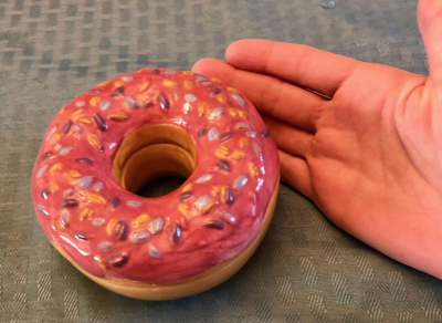
Please refer to the user guide for instructions on how to upload your pictures to the program to convert them to a 3D image. It also provides helpful tips on the angle you should take your pictures in order to best capture all the angles of the object or location you are using.
Here are a few tips for getting the best 3D image.
Any digital camera will work, including camera phones.
Save the photographs on the highest resolution and turn off any “live” features on the camera.
More than enough photographs of the object or setting is better than not enough.
Try to capture every angle or part of what you are photographing. It is okay if you miss a part of something as long as you capture it in another image.
Avoid using the flash and make sure you have good lighting.
Raw data converted to TIFF files work best, but you can also use JPG.
The program works with the original files, so do not crop, alter, or rotate any of the images before importing them into the program.
Creating your 3D Image in Structure from Motion
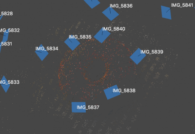
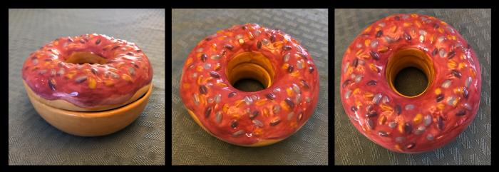
To create your 3D image, you will need to import the photographs and align them. Please refer to the user guide for step-by-step instructions and for help troubleshooting. After alignment, you will be able to see all the angle views plotted on the x, y, and z axes (Figure 16), and determine if you have photographed the object, landscape, etc. with enough coverage. It might be necessary to take new photographs if you determine that you are missing coverage in some areas.

The next steps are to build a dense point cloud and a mesh (Figure 17) based on the points generated in the point cloud. The dense point cloud image will look very similar to the image from the alignment step, but will probably contain more points. Creation of the mesh will fill in the space between the dots and will result in the 3D image. The time it takes to calculate and generate these will vary on the size of your object and/or landscape. The program created a dense point cloud of the ceramic donut that consists of over 9,000 individual points. After creating the mesh, you will be able to view your 3D image. The final 3D image of the ceramic donut contained almost 300,000 individual data points (Figure 17).
Transferability
Adaptations for Different K-12 Classrooms
The activity as described above is best suited for Middle and Upper Elementary School-aged children. However, simple adaptations can be made for students in High School. By engaging the students in more detailed discussions on climate change issues and engineering techniques, many of the Next Generation Science Standards for High School can be addressed. Younger age groups can simply work on manipulating the 3D printed models, helping them to make the connection between the model and an actual landscape. If it has been covered in school already, they can also work on taking measurements on the different parts of the 3D printed model.
Author/Credits
Lesson plan developed by Dr. Lauren Neitzke Adamo.
Data and technical support provided by Dr. Neal Iverson and Dr. Lukas Zoet.
Standards Other
Next Generation Science Standards (NGSS)
The following is a list of the Science and Engineering Practices, Crosscutting Concepts, and Core Disciplinary Ideas organized by a specific standard for Elementary and Middle School grades.
Elementary Standards
| Attachment | Size |
|---|---|
| Graph to use for creating mountain profiles. 302.4 KB | 302.4 KB |
| Emery 1961 paper on measuring beach profiles436.28 KB | 436.28 KB |
| STL file to 3D print the "Fully Assembled Mountain"3.01 MB | 3.01 MB |
| STL file to 3D print the "Puzzle Piece Mountain Part A"693.54 KB | 693.54 KB |
| STL file to 3D print the "Puzzle Piece Mountain Part B"756.63 KB | 756.63 KB |
| STL file to 3D print the "Puzzle Piece Mountain Part C"903.7 KB | 903.7 KB |
| STL file to 3D print the "Puzzle Piece Mountain Part D"707.6 KB | 707.6 KB |
| STL file to 3D print the "Puzzle Piece Mountain Part E"686.51 KB | 686.51 KB |
| 2nd Grade NGSS79.35 KB | 79.35 KB |
| 4th Grade NGSS81.67 KB | 81.67 KB |
| Middle School NGSS92.6 KB | 92.6 KB |
| STL file to 3D print the paper mount for the graphs.5.36 KB | 5.36 KB |
This program is supported by the National Science Foundation. Any opinions, findings, and conclusions or recommendations expressed by this program are those of the PIs and coordinating team, and do not necessarily reflect the views of the National Science Foundation.
